I always forget this, even though it’s super simple. So, I figured the best place to put it so that i would remember… is here in my blog. I use this a lot when I’m working on all kinds of spreadsheets, and I use spreadsheets constantly when I’m working on fonts, and with Adobe inDesign for data merges.
…but we’ll get to that later…
Here’s a quick formatting trick to highlight an entire row in Google Sheets.
Allow me to explain:
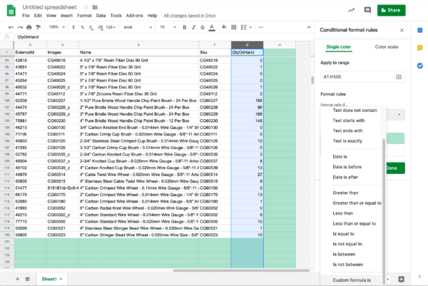
From the Sheets menu, select: Format > Conditional Formatting, and a dialog box will open on right side of your spreadsheet. For this example we’re just going to use “Single Color“, which should be the default.
For “Apply to range“, I’m going to apply it to the entire sheet starting at the first position, A1, and take it to the last row and column… which is H500 for this sheet. So, it will look like this:
A1:H500
Next, we’re going to want change “Format cells if…” by clicking on the drop down, and changing it to “Custom formula is“. This is where our formula comes in. For this sheet it is:
=$G1=0
What I’m doing here is having Sheets check to see if anything in column “G” has a value is equal to “0“. I’m applying it to row “1“, because that is the first row affected under “Apply to range” (A1:H500) directly above. These row numbers need match, or else the effected (affected?) rows will be offset, and it will look like your formula did not work.
Here’s a bit of back story (context) for anyone interested.
I was photographing products for a website, and needed to know what products were not in stock at the warehouse before I went searching for them. I used conditional formatting to hide any item that had a quantity of “0” on my printout.
So, here, instead of highlighting… I’m going to be changing the formatting of my cells that are out off stock to match the background color.
Ridiculously simple, but I always forget how to do this. So, now that I’ve written this I should hopefully remember.


