So, I’ve been tasked with sorting a bunch of data that all has to do with measurements… the only problem is, some of it is fractional, some of it is decimal, and some of it is metric. Which creates a couple of separate issues but right now I’m just going to talk about checking for a specific character in a cell.
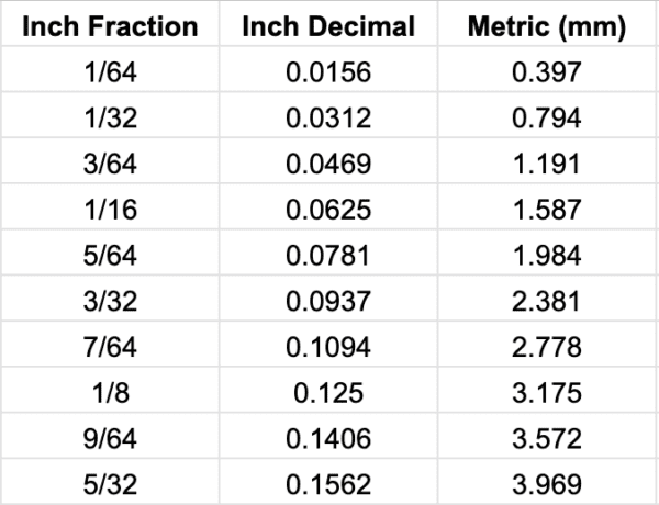
So, I’ve got this fancy chart for doing my conversions, and my plan is to use the FILTER function so that I can convert them all to decimal… because Sheets does some weird stuff with fractions. For this example I’m going to add the inch symbol to my fractional using this formula:
=A2&"""This returns the contents of cell A2, and adds the inch marker to the right, like so.
Perfect. Right? What about the fractions of less that 31 that could be easily read as dates?
Now we’re just going to take the visually simplest route to figure out which cells need fixed, because they all sort of blend together. I’m going to use this formula:
=IF(SEARCH("/",CELL),"","")You don’t need the IF function, I just wanted any cells that contained the forward slash to return no result. Anything that doesn’t will error out, like so…
So, now that we have those blocks sorted out we can use a different formula on them, to clear the year from their date formatting, and replace it with the inch mark.
=SUBSTITUTE(CELL,"/2020","")&""""Giving us the desired result… and fixing the #VALUE! error…
The story goes on from here, as I begin sorting my blend of Fractional, Decimal and Metric numbers, but I won’t bore you with that for now.


